
Okay, so check it out, I was messing around with some basketball data the other day, trying to figure out Kobe’s shot percentage.
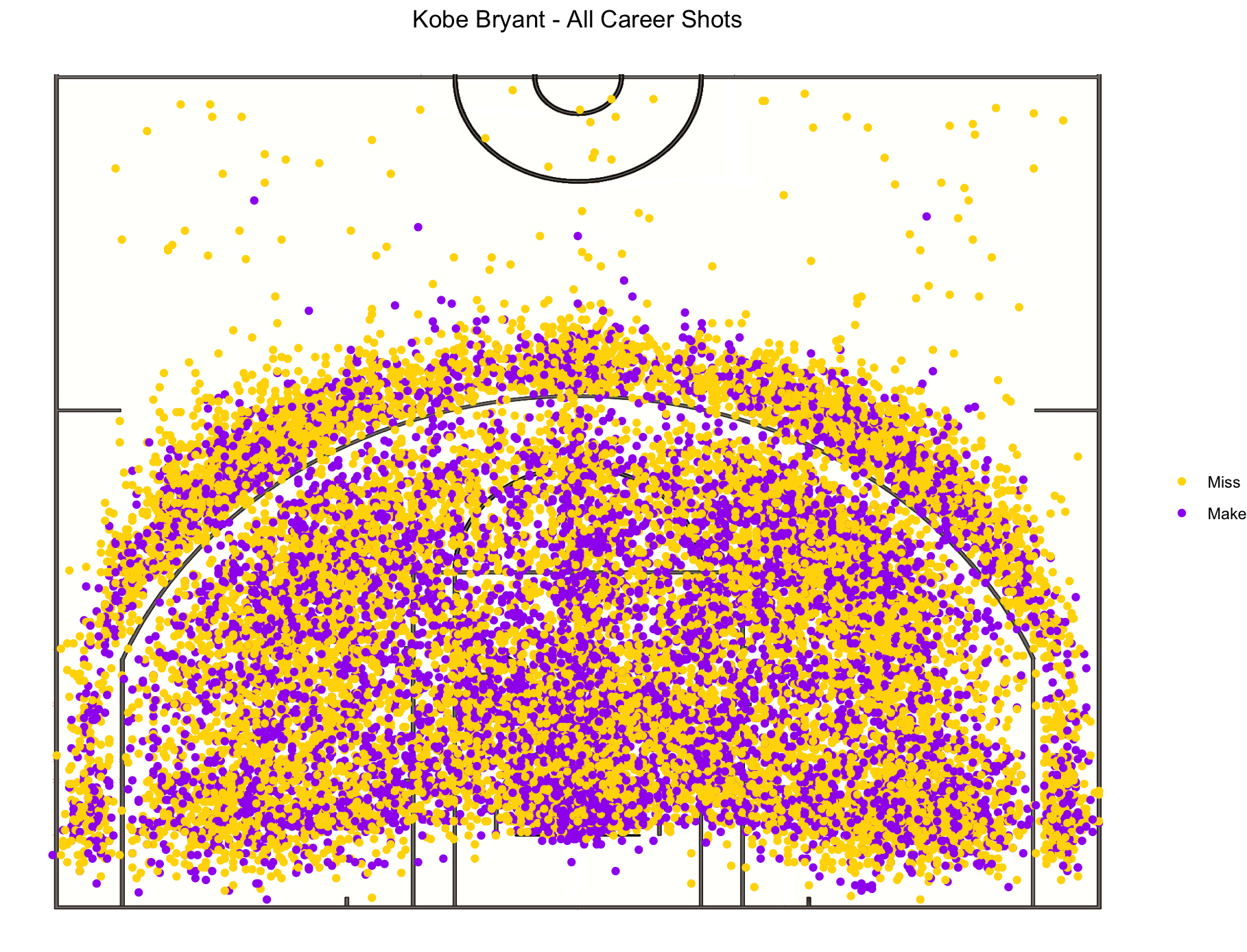
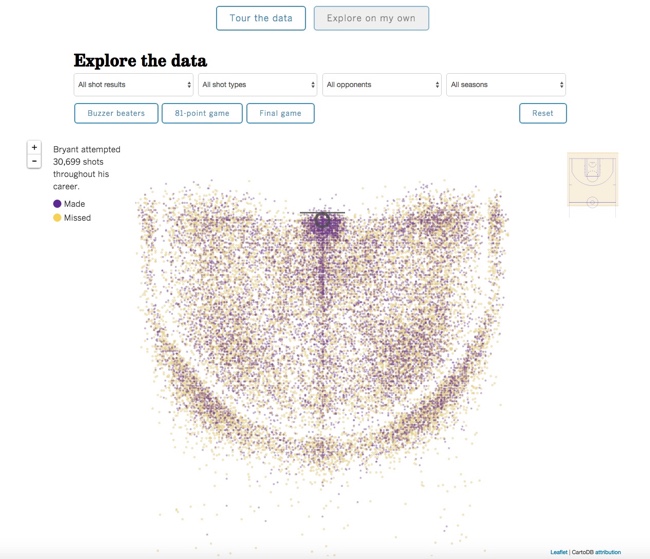
First, I started by hunting down a dataset. I found a pretty decent one on Kaggle that had details on every shot Kobe took in his career. Score!
Next up, I fired up my trusty Jupyter Notebook and loaded the data using pandas. I had to peek at the column names to figure out which one indicated whether a shot went in or not. Found it! It was something like ‘shot_made_flag’.
Then came the fun part. I used pandas to filter the dataframe and count how many shots he took in total, and how many he actually made. It was something like:
- total_shots = len(df)
- made_shots = df[‘shot_made_flag’].sum()
After that, I did the math. Simple division: made_shots / total_shots. That gave me his overall shooting percentage. I think it came out to be around 44% or something close. Not bad, Kobe!
But I wasn’t done yet. I wanted to see if his shooting percentage changed over the years. So, I grouped the data by season, and then calculated the shooting percentage for each season.
I plotted the results using matplotlib. It was cool to see how his shot percentage fluctuated throughout his career. Some seasons he was on fire, others, not so much.
Finally, I saved the results to a CSV file so I could show my friends. They were pretty impressed, especially when I showed them the plot of his shooting percentage over time.
It was a simple project, but it was a fun way to dig into some basketball data and learn a bit more about Kobe’s game. Plus, I got to practice my pandas and matplotlib skills. Win-win!


